Googling COVID-19: Supplementary Material
Greg Serapio-García
1 Preface
If you’re here from my poster at SPSP, you’ve come to the right place! This supplement will show how we are building longitudinal multilevel models for Google Search data related to coronavirus. The first example looks at search interest in cough symptoms; the second example examines all search interest related to the topic of coronavirus, in general.
Many thanks to my talented collaborators: Andrés Gvirtz, Elisa Militaru, Fritz Götz, Tobi Ebert, and Jason Rentfrow :)
This project remains exploratory and ongoing, please contact me with any questions or ideas for collaboration you may have!
(Skip to tl;dr/Discussion)
2 Introduction
Geographical variation in macropsychological traits predicts substantial political, economic, social and health outcomes (Rentfrow et al., 2013).
- Regional personality predicted economic resilience during the Great Recession of 2008—2009 (Obschonka et al., 2015).
- Regional personality predicted pandemic behavior at the onset of COVID-19 (Götz et al., 2020)
- Emerging research is also demonstrating how regional personality differences are influencing variation in COVID-19 infections and deaths (Peters et al., 2020)
- It therefore seems reasonable that geographical differences in personality would reflect variation in coronavirus-related Internet searches.
- Google Search data provide a aggregate measure of social thought and behavior recorded continuously over time. They can also be segmented at various geographical resolutions.
2.1 General Hypotheses
- Regions higher in conscientiousness, extraversion, and neuroticism will show a sharper increase in search interest for coronavirus.
- Regions lower in agreeableness will be slower to search for coronavirus.
3 Method
3.1 Overview
- Treat each region as an individual with repeated measurements of Internet search interest and time-invariant personality scores for N, E, O, A, C.
- Analyze these ‘individuals’ as if they were in an intensive longitudinal design. Intensive longitudinal data analyses prioritize investigation of both intra-individual and inter-individual change.
- Linear (and generalized!) multilevel models (MLMs) with time-invariant covariates
- (Also known as growth curve, latent curve, or hierarchical linear modeling)
- MLMs are super versatile: easy to customize covariance structures and nest participants within multiple groups, flexible time points
- c.f., conventional time series analyses are much more useful for prediction, rather than explanation
3.2 Data
- Regional personality data were taken from the Gosling-Potter Internet Personality Project.
- Google Search data came from:
- Google’s public-facing Trends website, which can be scraped with third-party R or Python packages.
- Returns search interest scores from 0 to 100 (continuous) scaled for a specified region, time restriction, and to most popular search term in a set of provided terms. 0 represents no search interest or not enough interest to preserve privacy. N.B.: Cannot directly compare search volume across regions or search terms, only changes in search.
- Google’s COVID-19 Symptoms Dataset (Public)
- Returns data in same format as above, meaning search volume across regions can’t be appropriately compared. Changes over time (i.e., trends) can be compared across regions, though.
- Can be called using BigQuery on Google Cloud Compute platform.
- Google’s Health Trends API (Private)
- Restricted access API that returns the estimated probability of searching a term for a given region and time restriction out of a stratified random sample all possible Google Searches, multiplied by 10 million for interpretability. Allows for comparisons of search volume across regions and time points. Differential privacy (i.e., from random sampling) slightly reduces reliability.
- To reduce measurement error and ensure replicability, it’s necessary to collect multiple samples of interest scores for a given search term.
- Google’s public-facing Trends website, which can be scraped with third-party R or Python packages.
3.3 Worked Example: Modeling Search Interest for Cough
This example uses Google’s public COVID-19 Symptoms Dataset.
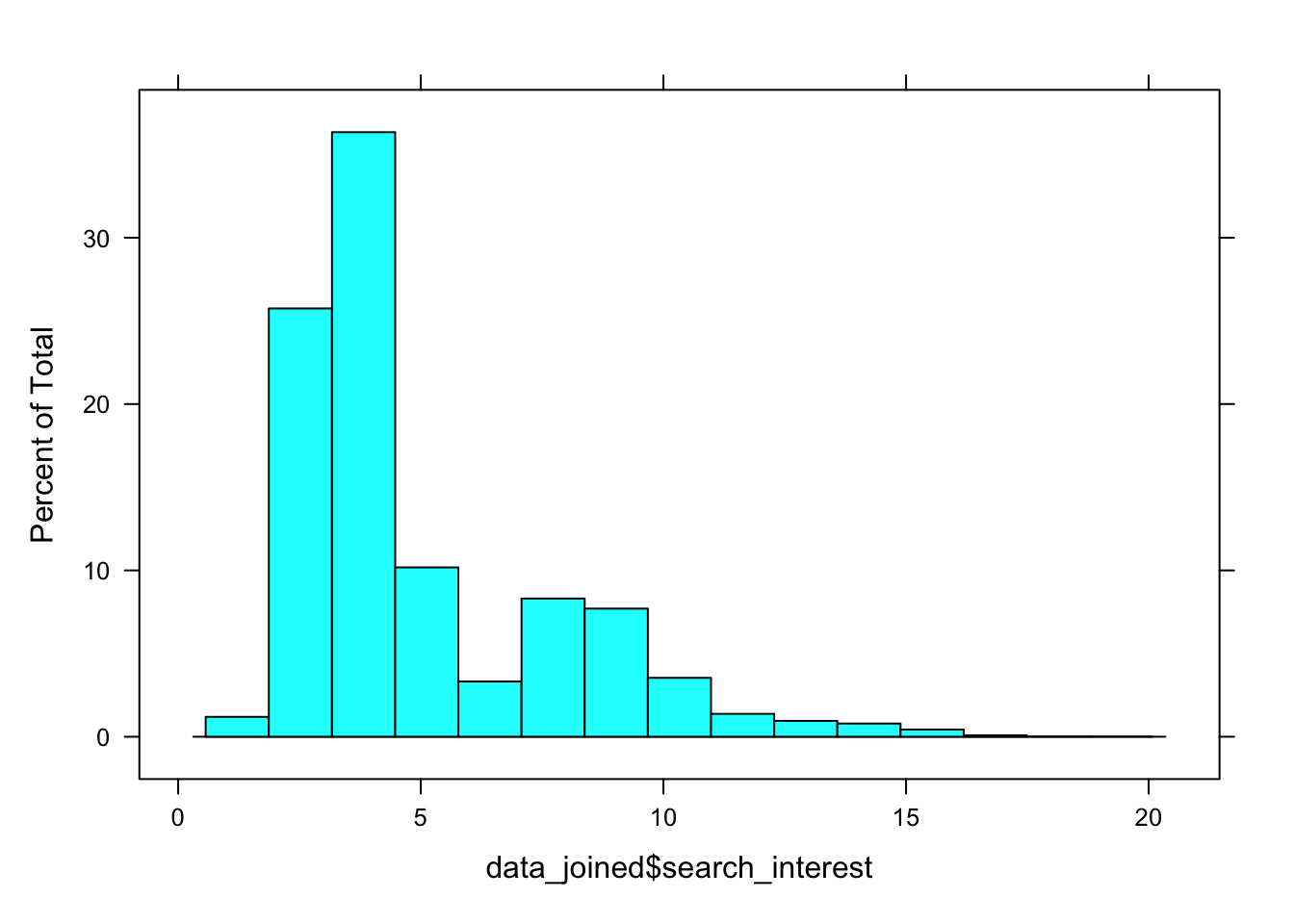
We can view the distribution of search interest scores (continuous, scaled from 0 to 100) for cough symptoms here. While the distribution isn’t zero-inflated, it’s overdispersed. For this reason, the search data for cough do not meet the normality criterion for multilevel linear modeling.
3.3.1 Predictive Power Score Analysis
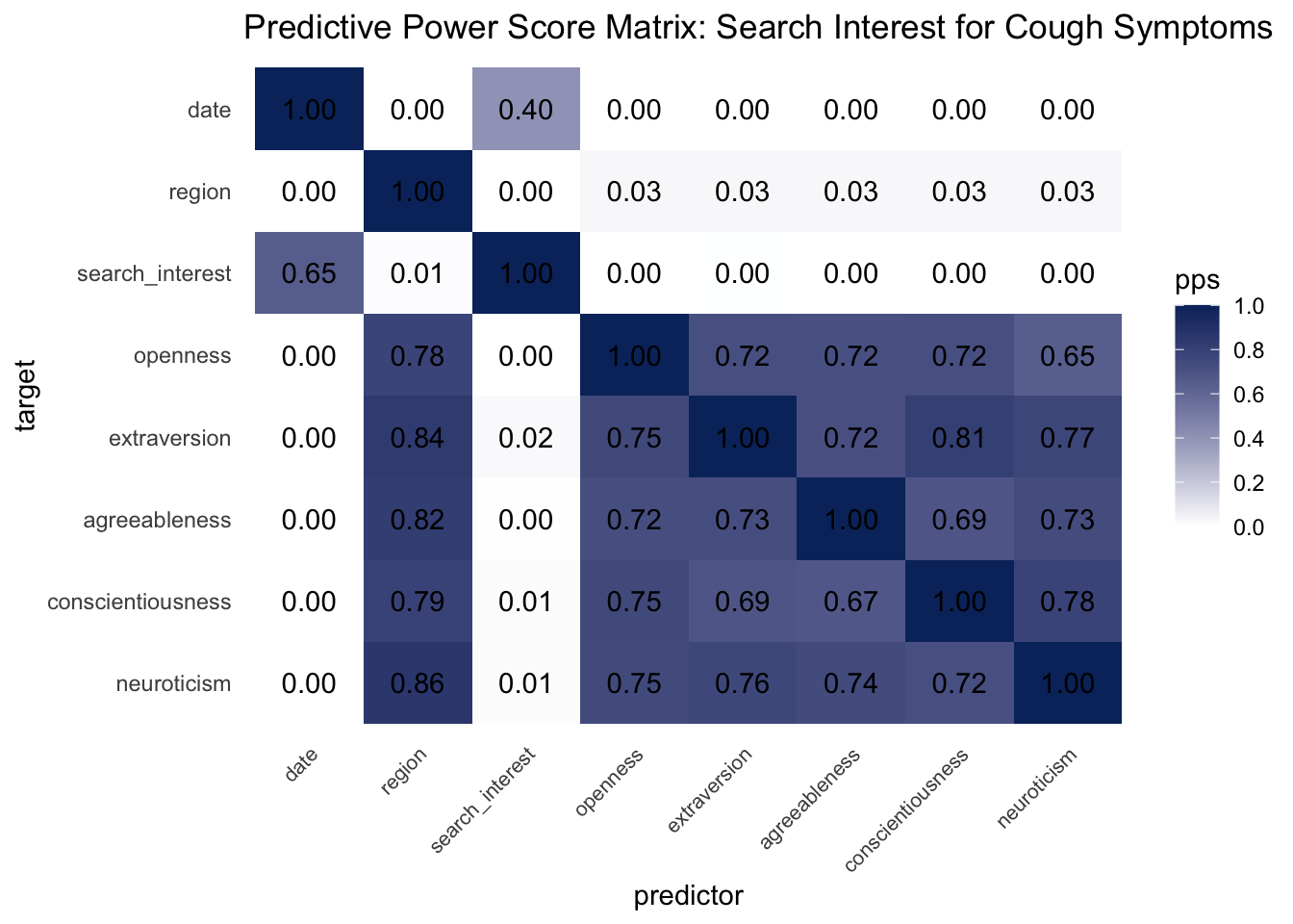
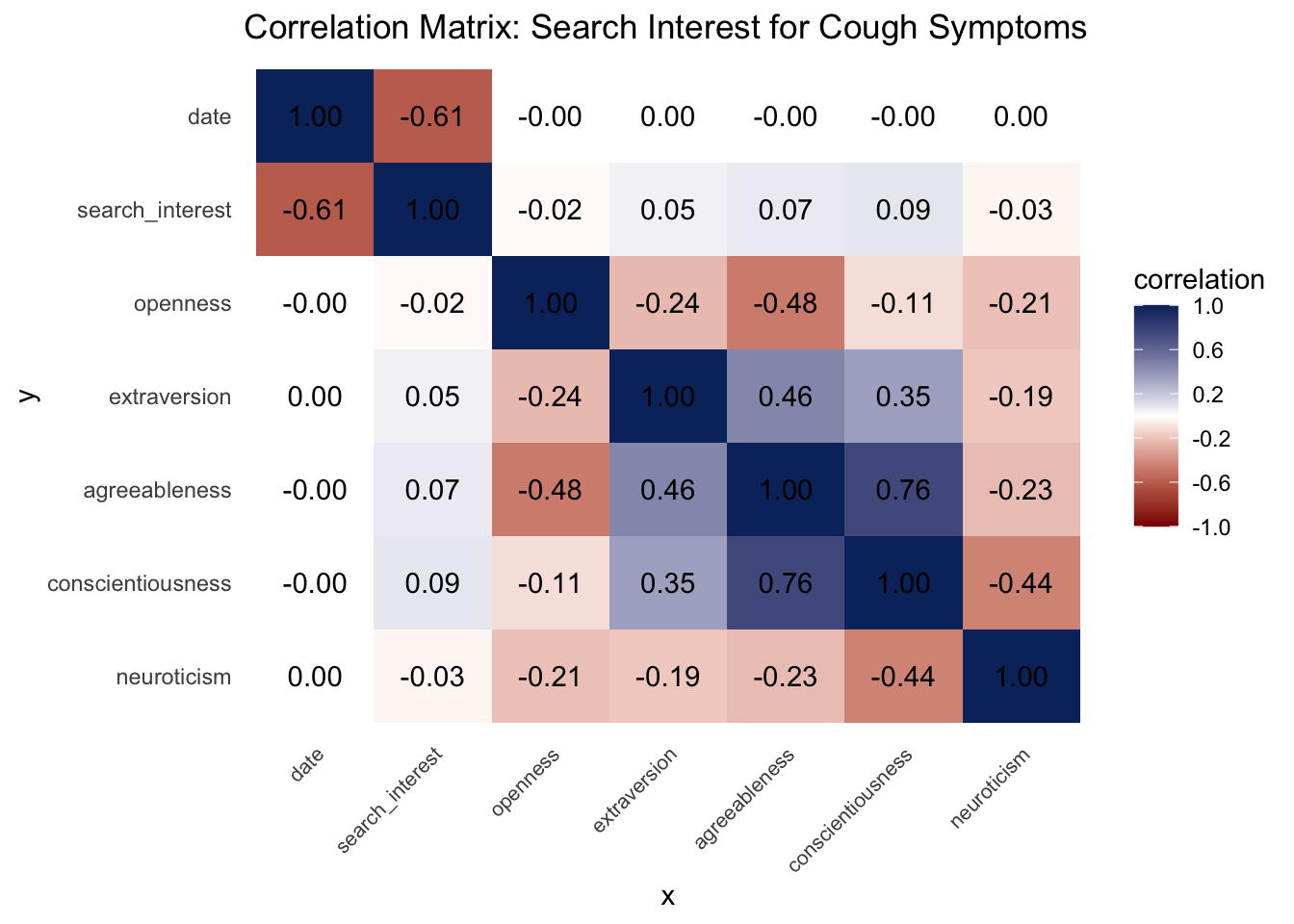
We can borrow some statistical rigor from machine learning to investigate the linear and non-linear predictive relationships between search interest and personality. Using a predictive power score (PPS) framework, we fit cross-validated decision trees and their normalized evaluation metrics for every bivariate combination of regional personality and search interest variables. PPS scores are data-type agnostic, so the distribution of cough interest isn’t an issue. Notice in the matrix visualization of PPS below that search interest in cough happens to predict personality, not the other way around!
3.3.2 Visualize Search Interest for Cough Symptoms Over Time
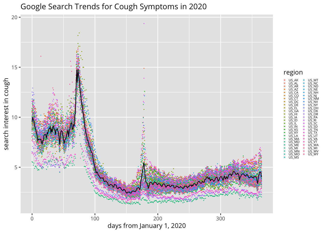
Double-click on a state’s abbreviation (on the right) to visualize its individual growth curve for cough-related search interest.
3.3.3 Build Multilevel Models
3.3.3.1 Random intercept model for quasi-poisson growth curves
- Tests whether initial levels of search interest (intercepts) by region are significantly different from each other. (We will have to ignore this model because these cough data happen to be scaled for each individual region, but this step definitely applies to production data taken directly from Google’s Health Trends API)
m0 <- glmmPQL(search_interest ~ 1,
              random = ~ 1 | region,
              family = quasipoisson(link = 'log'),
              data = data_joined)
## iteration 1## iteration 2## iteration 3summary(m0)## Linear mixed-effects model fit by maximum likelihood
## Data: data_joined
## AIC BIC logLik
## NA NA NA
##
## Random effects:
## Formula: ~1 | region
## (Intercept) Residual
## StdDev: 0.136 1.193
##
## Variance function:
## Structure: fixed weights
## Formula: ~invwt
## Fixed effects: search_interest ~ 1
## Value Std.Error DF t-value p-value
## (Intercept) 1.598 0.01945 18615 82.16 0
##
## Standardized Within-Group Residuals:
## Min Q1 Med Q3 Max
## -1.2045 -0.6772 -0.4353 0.7075 4.6908
##
## Number of Observations: 18666
## Number of Groups: 513.3.3.2 Random intercept + slopes quasi-poisson growth curves w/ time
- (We assume time will exert varying levels of influence on search interest among regions)
m1 <- glmmPQL(search_interest ~ date,
              random = ~ date | region,
              family = quasipoisson(link = 'log'),
              data = data_joined)
## iteration 1## iteration 2## iteration 3summary(m1)## Linear mixed-effects model fit by maximum likelihood
## Data: data_joined
## AIC BIC logLik
## NA NA NA
##
## Random effects:
## Formula: ~date | region
## Structure: General positive-definite, Log-Cholesky parametrization
## StdDev Corr
## (Intercept) 0.1208669 (Intr)
## date 0.0004323 0.09
## Residual 0.8230224
##
## Variance function:
## Structure: fixed weights
## Formula: ~invwt
## Fixed effects: search_interest ~ date
## Value Std.Error DF t-value p-value
## (Intercept) 2.1348 0.017583 18614 121.42 0
## date -0.0033 0.000066 18614 -49.49 0
## Correlation:
## (Intr)
## date -0.01
##
## Standardized Within-Group Residuals:
## Min Q1 Med Q3 Max
## -1.79238 -0.72305 -0.05586 0.65527 6.60049
##
## Number of Observations: 18666
## Number of Groups: 513.3.3.3 Random coefficient quasi-poisson growth curves
- We add in regional personality traits as time-invariant covariates exerting influence on levels of search.
m2 <- glmmPQL(search_interest ~
                extraversion +
                agreeableness +
                conscientiousness +
                neuroticism +
                openness +
                date,
              random = ~ date | region,
              family = quasipoisson(link = 'log'),
              data = data_joined)
## iteration 1## iteration 2## iteration 3summary(m2)## Linear mixed-effects model fit by maximum likelihood
## Data: data_joined
## AIC BIC logLik
## NA NA NA
##
## Random effects:
## Formula: ~date | region
## Structure: General positive-definite, Log-Cholesky parametrization
## StdDev Corr
## (Intercept) 0.1190034 (Intr)
## date 0.0004352 0.025
## Residual 0.8230438
##
## Variance function:
## Structure: fixed weights
## Formula: ~invwt
## Fixed effects: search_interest ~ extraversion + agreeableness + conscientiousness + neuroticism + openness + date
## Value Std.Error DF t-value p-value
## (Intercept) 2.1348 0.0173 18614 123.15 0.0000
## extraversion 0.6302 0.6891 45 0.91 0.3653
## agreeableness 0.2520 0.9125 45 0.28 0.7837
## conscientiousness 0.0151 0.9854 45 0.02 0.9878
## neuroticism 0.2089 0.5443 45 0.38 0.7029
## openness 0.4154 0.4216 45 0.99 0.3297
## date -0.0033 0.0001 18614 -49.20 0.0000
## Correlation:
## (Intr) extrvr agrbln cnscnt nrtcsm opnnss
## extraversion -0.001
## agreeableness 0.000 -0.244
## conscientiousness -0.001 0.023 -0.747
## neuroticism 0.000 0.117 -0.026 0.308
## openness 0.000 0.059 0.555 -0.325 0.247
## date -0.069 0.002 -0.001 0.002 0.000 0.000
##
## Standardized Within-Group Residuals:
## Min Q1 Med Q3 Max
## -1.79073 -0.72305 -0.05492 0.65442 6.60218
##
## Number of Observations: 18666
## Number of Groups: 513.3.3.4 Final model: Random coefficient quasi-poisson growth curves + interaction w/ time
- We allow regional personality to interact with time, which shows how personality affects both levels and rates of search interest across regions.
m3 <- glmmPQL(search_interest ~
                (extraversion +
                   agreeableness +
                   conscientiousness +
                   neuroticism +
                   openness) * (date),
                random = ~ date | region,
                family = quasipoisson(link = 'log'),
                data = data_joined)
## iteration 1## iteration 2## iteration 3summary(m3)## Linear mixed-effects model fit by maximum likelihood
## Data: data_joined
## AIC BIC logLik
## NA NA NA
##
## Random effects:
## Formula: ~date | region
## Structure: General positive-definite, Log-Cholesky parametrization
## StdDev Corr
## (Intercept) 0.1190490 (Intr)
## date 0.0002118 0.109
## Residual 0.8232172
##
## Variance function:
## Structure: fixed weights
## Formula: ~invwt
## Fixed effects: search_interest ~ (extraversion + agreeableness + conscientiousness + neuroticism + openness) * (date)
## Value Std.Error DF t-value p-value
## (Intercept) 2.1347 0.0173 18609 123.10 0.0000
## extraversion 0.6100 0.6912 45 0.88 0.3822
## agreeableness 0.3463 0.9150 45 0.38 0.7069
## conscientiousness -0.2068 0.9880 45 -0.21 0.8352
## neuroticism 0.2402 0.5458 45 0.44 0.6620
## openness 0.4978 0.4228 45 1.18 0.2452
## date -0.0033 0.0000 18609 -82.11 0.0000
## extraversion:date 0.0007 0.0016 18609 0.46 0.6451
## agreeableness:date -0.0056 0.0021 18609 -2.65 0.0080
## conscientiousness:date 0.0138 0.0023 18609 6.11 0.0000
## neuroticism:date -0.0012 0.0013 18609 -0.98 0.3265
## openness:date -0.0047 0.0010 18609 -4.83 0.0000
## Correlation:
## (Intr) extrvr agrbln cnscnt nrtcsm opnnss date extrv:
## extraversion -0.001
## agreeableness 0.000 -0.244
## conscientiousness -0.001 0.023 -0.747
## neuroticism 0.000 0.117 -0.025 0.308
## openness 0.000 0.059 0.555 -0.325 0.247
## date -0.072 0.003 -0.001 0.004 0.000 0.000
## extraversion:date 0.003 -0.081 0.023 -0.005 -0.005 -0.002 -0.009
## agreeableness:date -0.001 0.023 -0.073 0.054 -0.001 -0.039 0.006 -0.258
## conscientiousness:date 0.004 -0.005 0.054 -0.068 -0.018 0.022 -0.018 0.037
## neuroticism:date 0.000 -0.006 -0.001 -0.018 -0.073 -0.021 0.000 0.108
## openness:date 0.000 -0.002 -0.039 0.022 -0.021 -0.073 0.007 0.052
## agrbl: cnscn: nrtcs:
## extraversion
## agreeableness
## conscientiousness
## neuroticism
## openness
## date
## extraversion:date
## agreeableness:date
## conscientiousness:date -0.753
## neuroticism:date -0.019 0.298
## openness:date 0.552 -0.327 0.253
##
## Standardized Within-Group Residuals:
## Min Q1 Med Q3 Max
## -1.79025 -0.72459 -0.05383 0.65274 6.57886
##
## Number of Observations: 18666
## Number of Groups: 513.3.4 Visualize estimated interactions w/ time (how personality affects rate of search interest)
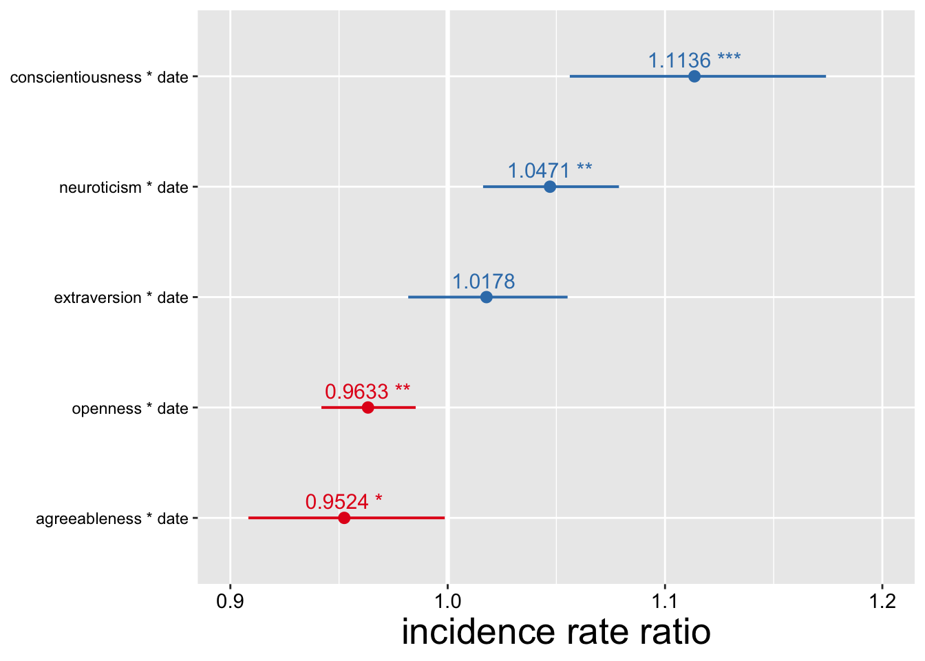
plot_TICs(data_joined, "search_interest") + ylim(.99, 1.02) + labs(title = "Estimated Personality Effects on Search Trends for Cough")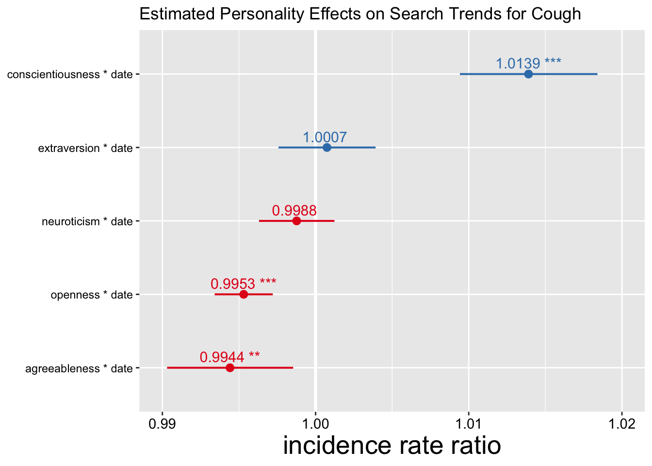
- Interpretation: for every standard deviation increase in regional conscientiousness, rate of change in search interest for cough symptoms increases by an estimated factor of 1.0139.
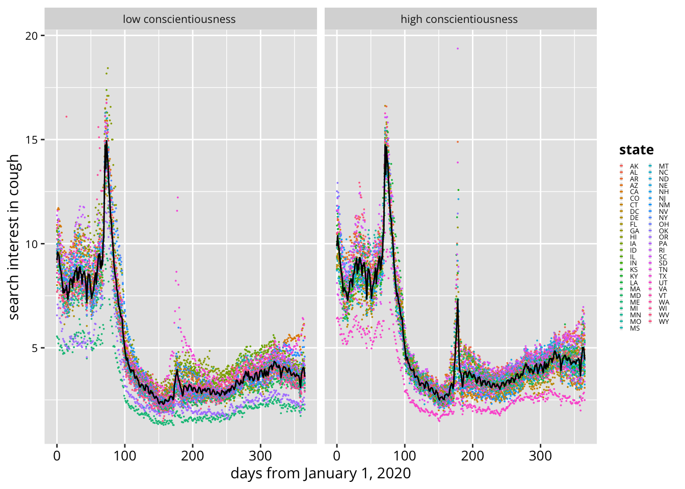
3.3.5 Compare growth curves of search interest by state levels of conscientiousness
4 Results and Discussion
4.1 tl;dr:
- In these initial models of COVID-related Google Search trends, regional differences in personality are surprisingly important—even without controls for statistical noise and regional demographics. Aggregate conscientiousness appears to be the primary driver of coronavirus-related searches over time.
- Possible explanation: High C regions are more diligent, dutiful about looking out for COVID-19 symptoms, guidelines, news.
4.2 Summary of Preliminary Results
- Hypothesis 1: supported by these preliminary models. Visualization of coronavirus model shows the positive influence of C, N, and E on COVID-19-related search interest.
- Hypothesis 2: mixed support. Low A predicts slower interest in cough symptoms but is not significantly related to coronavirus search volume in general.
4.4 Implications
- Further evidence: Macropsychological traits influence aggregate behavior, particularly in times of crisis
- Regions lower in C might need extra promotion of COVID-19 related information
- Regions higher in C will probably show lower rates of infection and higher adherence to guidelines (we’re seeing preliminary evidence of this in the literature)
4.5 Limitations / Next Steps
- In general, we need to examine more specific search behaviors to rule out search scenarios in which personality traits have diverging influence.
- For example: searches related to “cough” may be popular among high C regions out of dutifulness, but also among low C regions out of carelessness.
- Does search interest for these terms indicate compliance, or non-compliant behaviors which have led to infection?
- Choosing a proper distribution for continuous data that’s sometimes zero-inflated. Gamma? Quasi-poisson?
- What are the underlying assumptions of generalized multilevel models for these distributions?
- Why does search interest more strongly predict personality in exploratory analyses rather than the other way around?
- Could this be for certain traits only?
- To-Do: Incorporate temporal and spatial autocorrelation in generalized MLMs
- To-Do: Poststratify/adjust estimates by region population
- To-Do: Incorporate additional levels of geographical resolution into the same models: counties can be nested in metro DMAs which can be nested in states
